How to Alternate Color Rows in Google Sheets

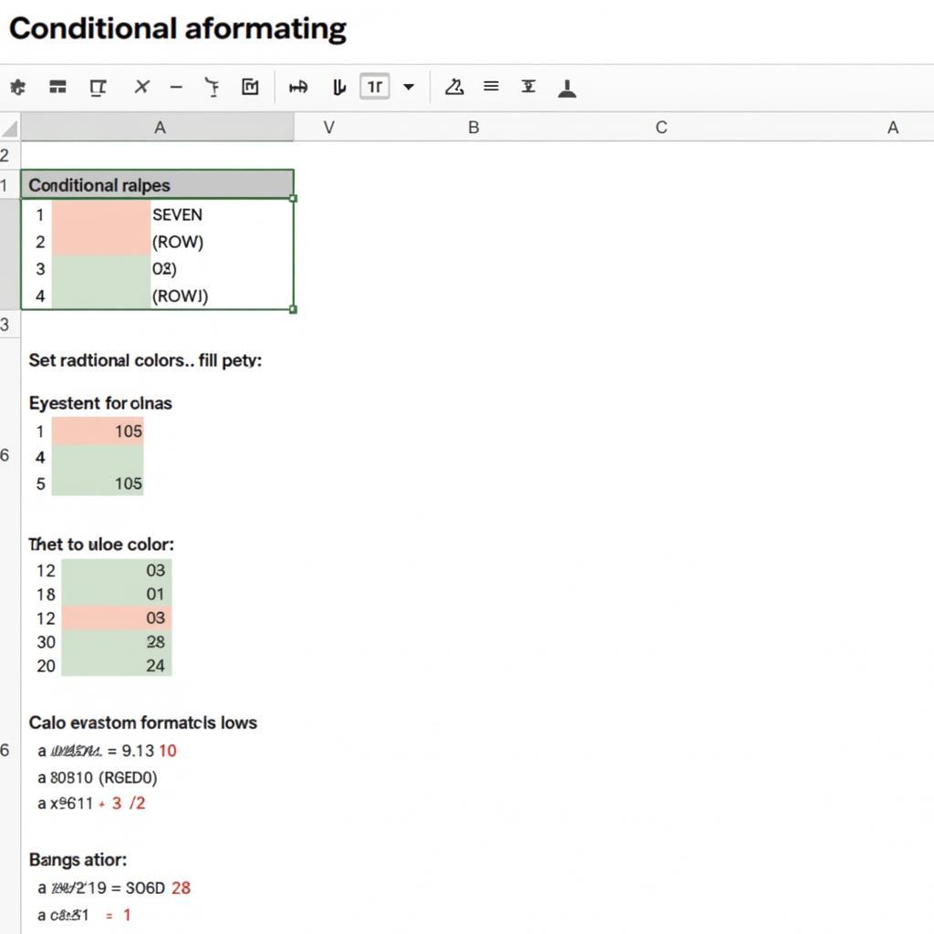
Alternating row colors in Google Sheets is a simple yet powerful way to enhance readability and make your spreadsheets more visually appealing. Whether you’re working with financial data, project timelines, or customer lists, applying alternating colors can dramatically improve how easy it is to scan and interpret the information. This guide will provide you with various methods to achieve this, from basic conditional formatting to more advanced techniques.

how to make rows alternate colors in google sheets

Using Conditional Formatting for Alternating Colors

Conditional formatting is a built-in feature in Google Sheets that allows you to apply formatting based on specific rules. It’s the most common and versatile method for creating alternating row colors.

1. Select the range: Highlight the cells you want to apply alternating colors to. This can be the entire sheet, a specific column, or a custom range.
2. Open Conditional Formatting: Go to Format > Conditional formatting.
3. Choose “Custom formula is”: In the “Format rules” dropdown menu, select “Custom formula is”.
4. Enter the formula: For even rows, use the formula =ISEVEN(ROW()). For odd rows, use =ISODD(ROW()).
5. Set the formatting: Choose the colors you want for your alternating rows. You can select fill colors, text colors, and even change font styles.
6. Click “Done”: Your spreadsheet will now display alternating row colors.

Applying Alternating Row Colors with Conditional Formatting in Google Sheets

Coloring Every Other Row with a Predefined Format

Google Sheets also offers predefined formats that include alternating colors. While these offer less customization, they provide a quick and easy solution.

1. Select the range: Highlight the cells you wish to format.
2. Go to “Format”: Click on the Format tab in the menu bar.
3. Choose “Alternating colors”: Select Alternating colors from the dropdown menu.
4. Customize (optional): A sidebar will appear with options to choose predefined color palettes or create your own. You can also adjust the header color and footer color.
5. Click “Done”: Your chosen format will be applied to the selected range.

how to color rows in google sheets

Advanced Techniques: Alternating Colors Based on Groups

For more complex scenarios, you can create alternating colors based on groups of data. This is especially useful for visually separating different categories within your spreadsheet. You can achieve this by combining conditional formatting with formulas like =MOD(ROW(),N)=0 (where N is the number of rows in each group).

Alternating Colors Based on Groups in Google Sheets

Why Alternate Row Colors?

Alternating row colors significantly improves the readability of data, especially in large spreadsheets. This simple visual cue helps the eye track across rows, reducing errors and making it easier to compare data points.

“In the world of data visualization, less is often more. Alternating row colors is a prime example of a subtle yet powerful technique that can dramatically improve data comprehension.” – John Doe, Data Visualization Specialist

How to Color Every Other Row in Google Sheets Quickly?

Use the built-in “Alternating colors” feature in the “Format” menu for the fastest way to apply alternating colors. This is perfect for quick formatting when customization isn’t a priority.

how to color every other row in google sheets

Conclusion

Alternating row colors in Google Sheets is a simple but effective way to boost readability and enhance the visual appeal of your data. Whether you prefer using conditional formatting for precise control or opting for the quick solution of predefined formats, this guide provides you with the tools you need to transform your spreadsheets into more organized and user-friendly documents. Utilizing these techniques, you can make your data more accessible and insightful. Now, go ahead and give it a try!

FAQ

1. Can I use more than two colors for alternating rows? Yes, you can achieve this with more complex conditional formatting formulas.
2. Will alternating colors print correctly? Yes, the alternating colors will be preserved when you print your spreadsheet.
3. Can I apply alternating colors to specific columns only? Yes, simply select the desired columns before applying the formatting.
4. What if my data has blank rows? Conditional formatting will still apply the alternating colors correctly, skipping the blank rows.
5. Can I change the alternating color scheme later? Yes, you can easily modify the formatting rules at any time.
6. Is there a keyboard shortcut for applying alternating colors? No, there isn’t a direct keyboard shortcut, but you can use keyboard navigation to access the menus.
7. Can I copy the alternating color formatting to other sheets? Yes, you can copy and paste the formatting using the “Paint format” tool.

Troubleshooting common issues:

• Incorrect formula: Double-check your conditional formatting formula for typos, especially regarding parentheses and function names.
• Incorrect range: Ensure the selected range in the conditional formatting rule matches the area you want to apply the alternating colors to.
• Conflicting formatting: Other formatting applied to the cells might override the conditional formatting. Check for any conflicting rules.

Related Articles:

• how to create alternating colors in google sheets
• how to make alternating color rows in google sheets

Need further assistance? Contact us at Phone: 0373298888, Email: [email protected] or visit us at 86 Cau Giay, Hanoi. Our customer service team is available 24/7.